Results
Denoising:
In the images above, we see a number of waveforms. Each image has three waveforms: an original waveform, a waveform with added noise, and a denoised waveform. From these examples, we can learn much about our approach to denoising. In the first image, we see a very smooth-looking waveform with a small amount of noise added. We observe that the denoising process leaves the signal slightly less smooth than before, but does a good job of maintaining the overall shape of the original signal. Thus, we understand that our denoising process does well when the signal to noise ratio is high, with very little loss in quality.
In the second image, we see a limitation of our denoising process. The noise added is much larger than the weak signal, so after the denoising process, the shape of the signal has changed dramatically. However, the signal is still relatively smooth after denoising, so our denoising process does a good job of reducing the variance of a signal due to noise. This would correspond to an improvement in sound quality in some contexts.
In the last 3 images, we note a variety of effects of denoising. We see that parts of signals with very low amplitude are not preserved well by the denoising process. We also see that even a signal that oscillates wildly (such as the final image) is preserved fairly well by the denoising process. An overly naive denoising method might collapse the last signal completely in denoising, but our denoising process is able to precisely identify the amount of variance to remove from a signal.
Above we have 3 spectrograms and 3 audio tracks. The first of each corresponds to a short piece of audio recorded on a piano. The second results from adding noise to the signal. The third results from applying our denoising process. The noise manifests itself as an abundance of light spots on the upper part of the second spectrogram. In the audio, we hear the noise as white noise or static. After denoising, we can still notice some of these spots or static, but much of it is gone.
This demonstration gives us a mapping from the waveforms we observed earlier to the spectral domain and human hearing. We observe a link between the small jaggedness introduced by noise, the light spots on the spectrogram, and the white noise in the audio. Essentially, white noise is small, rapid oscillations in the audio track, spread across many pitches. Thus, we find that perceived audio quality is directly affected by our ability to minimize and smooth out these oscillations.
This demonstration gives us a mapping from the waveforms we observed earlier to the spectral domain and human hearing. We observe a link between the small jaggedness introduced by noise, the light spots on the spectrogram, and the white noise in the audio. Essentially, white noise is small, rapid oscillations in the audio track, spread across many pitches. Thus, we find that perceived audio quality is directly affected by our ability to minimize and smooth out these oscillations.
Auto-Tuning with Phase-Vocoder:
Above we have three plots that help illustrate some of the phase-vocoder process. The first plot is that of the frequency-domain representation of an input song at a single moment in time. We see a number of peaks at different points on the frequency spectrum. These peaks represent the prominent pitches in the song at this time step. These peaks also have regions of influence which can be defined by dividing the regions between adjacent peaks in half. By shifting these peaks along with their regions of influence, we can modify the perceived pitch of a song. It's important to note that some of these peaks do not represent "true" pitches in the music. Peaks can be caused by harmonics and can also be induced by the side lobes of the windowing function used for the STFT. However, phase-vocoding does provide the opportunity to manipulate individual peaks so that individual voices in a multitrack recording can be pitch adjusted.
In the second image, we see a frequency spectrum before and after shifting peaks. Because we are moving pitches to the nearest frequencies, we often do not have to shift their frequencies by very much. Thus, the shifted spectrum looks very similar to the original spectrum.
In the last image, we show a sine wave before and after a frequency adjustment of 1.1 times. We see that the right end of the sine waves no longer line up. If we naively apply frequency shifting to an entire audio sample, we will find that the phases at each timestep do not line up. To remedy this, we apply a phase shifting factor, which is a complex exponential of the frequency shift we applied. This allows the phases to match up and improves the sound quality.
Here we see the result of applying a phase vocoder to pitch shift a short singing sample (both a spectrogram and an audio file). Our STFT used a hanning window with a 1 second width, a 0.5 second step size, and a 1024 point FFT. After some failed attempts at manipulating various types and numbers of peaks, we settled on manipulating the maximal peak for the best sound quality. Unfortunately, the quality of the resulting clip was not very good. We can see in the spectrogram of the output that certain frequency bands are almost completely absent. This may be an artifact of representing the frequency domain with discrete frequency bins.
We suspect that the sampling rate and window shape of our STFT may be having a negative effect on the output sound quality. However, trying to use denser windows (larger width with smaller step size) or more points in our FFT slows down computation significantly. As a result, it seems we need to be more clever about maintaining sound quality if we want our phase-vocoder implementation to be useful for real-time applications. We lastly note that while the pitch correction works when the singer sings some notes out of tune, if the notes are too out of tune, the pitch correction fails to find the correct pitch. This is expected from not using a ground truth to compare to. Without a much more sophisticated method, it is hard to do better than snapping sounds to their closest pitch.
We suspect that the sampling rate and window shape of our STFT may be having a negative effect on the output sound quality. However, trying to use denser windows (larger width with smaller step size) or more points in our FFT slows down computation significantly. As a result, it seems we need to be more clever about maintaining sound quality if we want our phase-vocoder implementation to be useful for real-time applications. We lastly note that while the pitch correction works when the singer sings some notes out of tune, if the notes are too out of tune, the pitch correction fails to find the correct pitch. This is expected from not using a ground truth to compare to. Without a much more sophisticated method, it is hard to do better than snapping sounds to their closest pitch.
Other Auto-Tuning Methods:
For the remaining experiments, we primarily focus on the two audio clips represented above. The first clip is a piano audio clip with a number of out of tune notes. The second clip is a ground truth, which we can compare our results to, and in many cases, even fit our pitches by directly using it.
Above is the output of 4 different Auto-Tuning algorithms in both spectrogram and audio form. The first algorithm tunes the audio without a ground truth using a thresholding method. All frequencies above a given threshold are snapped to the nearest pitch on a 12-tone scale. This has an advantage over phase-vocoding because it is relatively simple and computationally inexpensive. However, it degrades the timbre of the sound by collapsing all frequencies above a certain threshold to fixed pitches. We can hear this damage to the audio quality in the recording, which has a somewhat unpleasant grinding sound in the background. Furthermore, this technique does not bring the pitches to our actual target ground truth. After all, it does not even know what the target ground truth is.
The second algorithm tunes the audio in a column-wise fashion. That is each individual time step is analyzed and each frequency component is shifted to match the ground truth frequency on a point-by-point basis with some smoothing done to improve audio quality. Thus, this algorithm manifests as "smearing" the columns, relative to the other methods, which leave clear horizontal lines corresponding to held notes. Unfortunately, manipulating the audio on such a fine-grained basis destroys almost all of the natural quality of the sound. While it sounds closer to the ground truth in terms of pitch, the piano is unrecognizable.
The third algorithm tunes the audio in a segment-wise fashion. The audio is segmented at regular intervals identified by changes in sound intensity, representing notes. The ground truth frequency is tested over these intervals, and the entire segments of the spectrogram are shifted accordingly. We see this manifest as having clearly segmented rows in the spectrogram. We can hear that this method preserves much of the original timbre of the piano sound. However, it does a much worse job of extracting the pitch of the ground truth. It may be necessary to combine this segment-wise method a better method of pitch detection for the ground truth. Additionally, the segment-wise method requires identifying hop sizes based on sound intensity, which means that some types of music which are do not have note boundaries easily detected by this method may not be tuned well.
The fourth algorithm tunes the audio in a pitch-wise fashion. Once again the audio is segmented, but now the whole columns are shifted up or down in unison. Interestingly, the quality of this sound seems to be worse than the third algorithm, despite the fact that horizontal segments are not being manipulated. However, it seems to be slightly closer to properly tuning the pitches than the segment-wise algorithm.
From these experiments, we see that, while fine-grained control over frequencies and sounds can help to match pitches, a holistic approach to pitch modification is necessary to preserve sound quality. Future approaches to this problem would likely involve grouping nearby frequencies to move in order to preserve the shape of the frequency spectrum.
PSOLA-based autotuning:
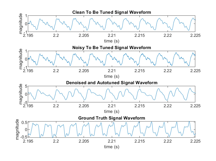
Our final experiment combines denoising with the PSOLA method for Auto-Tuning. We added noise to our original audio, de-noised it, and then used PSOLA to Auto-Tune it to our ground truth. Interestingly, we can see that the total peaks in the observing window changes between to-be-tuned signal and Auto-Tuned signal. In fact, before tuning there are 10 peaks. After tuning, there are 13 peaks which is the same as ground truth. Although these peaks are not perfectly periodic, they sound right.
Essentially, the PSOLA method has been our most successful method of Auto-Tuning. It maintains some of the natural timbre of the sound (although not much), but it does a very good job of matching the pitches of the ground truth. The song is easily recognizable in the output. In the future, we may want to pursue improvements on the PSOLA method in order to improve the sound quality and handle some of the grating sounds introduced in the audio as a result of processing with this algorithm.
Essentially, the PSOLA method has been our most successful method of Auto-Tuning. It maintains some of the natural timbre of the sound (although not much), but it does a very good job of matching the pitches of the ground truth. The song is easily recognizable in the output. In the future, we may want to pursue improvements on the PSOLA method in order to improve the sound quality and handle some of the grating sounds introduced in the audio as a result of processing with this algorithm.