Background
Humans perceive sound when sound waves hit the eardrum. This causes the eardrum to vibrate according to the frequency of the sound. The higher the frequency of a sound, the higher the perceived pitch. The volume of the sound is determined by the amplitude of the vibrations. A song is simply combinations of different frequencies and amplitudes happening at different times. We are not directly concerned with volume, although it is important to keep the volume of a sound at a reasonable level when doing de-noising or pitch correction.
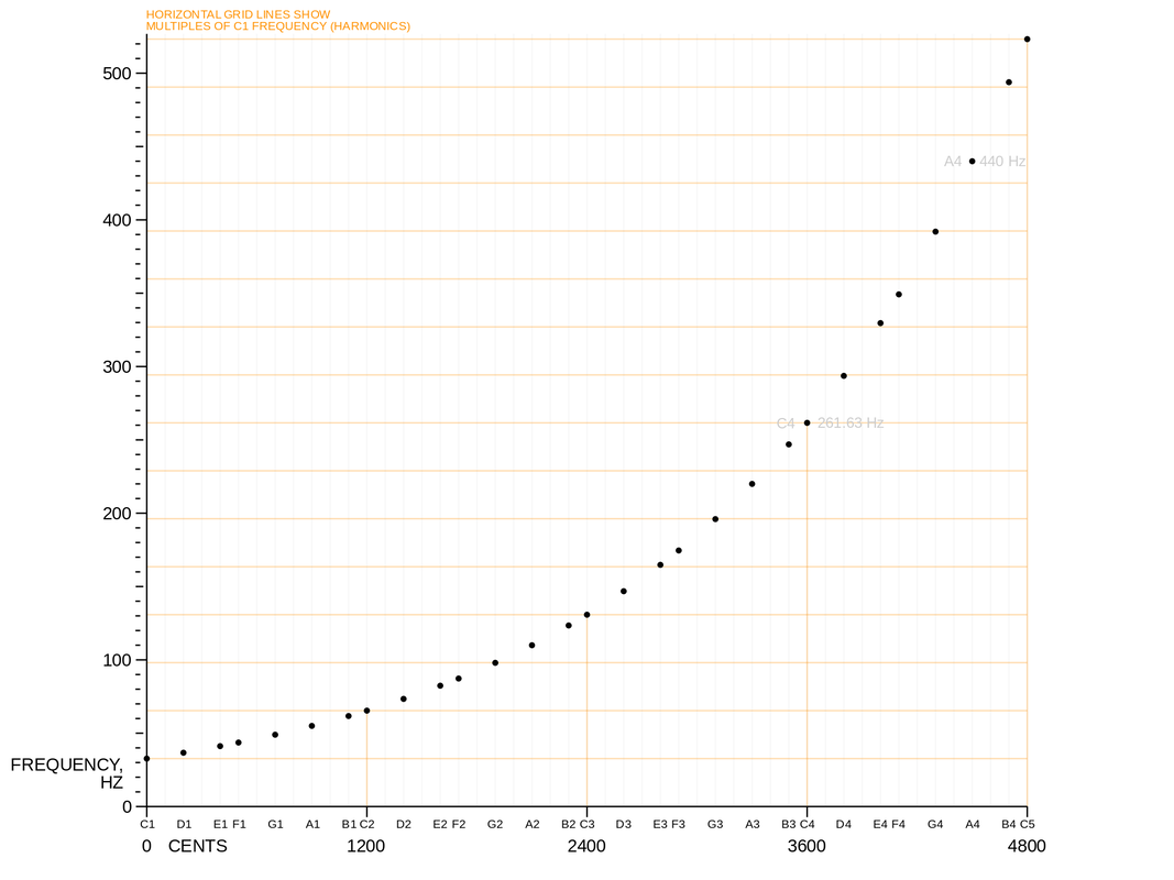
Musical pitches can be modeled as a discrete set of frequencies. Humans perceive pitch logarithmically, so natural divisions of pitches are determined by fixing the ratio between pitches. Notably, many people perceive pitches with a whole number ratio as being "identical." The smallest nontrivial whole number ratio is 2, and pitches with a ratio of 2 are called an "octave." The most standard musical scale is the 12-tone scale, which subdivides an octave into 12 evenly spaced pitches. This means that consecutive pitches are separated by a factor of 21/12. The 12-tone scale has been chosen because many pairs of pitches in the scale have ratios which are well-approximated by rational numbers with small denominators.
Theoretically, singers and musicians should perform these pitches exactly; for example, 'do' in C major is 261.6Hz, 're' in C major is 293.6Hz. Of course, no one can always be exactly on the right pitch. Many great singers may be "almost right" most of the time so that people cannot detect the difference. Less practiced individuals are likely to be noticeably different from the standardized set of pitches.
To correct pitches in music, we divide the task into several parts, namely De-noising, Frequency Detection, Pitch Correction, and Smoothing.
Frequency of pitch
Frequency Detection:
STFT:
As we stated earlier, pitch is determined by the frequency of a sound. In order to detect pitch, we need to convert audio signals from the time domain to the frequency domain. The commonly used Discrete Fourier Transform (FFT in MATLAB) operates over the entirety of a finite length signal. This does not give us a reasonable interpretation of a signal’s frequency at a specific time. Importantly, it does not allow us to extract the different pitches throughout the duration of a song. To remedy this, we use the Short Time Fourier Transform (STFT). The STFT samples the signal at different timesteps using a windowing function and then applies a Discrete Fourier Transform (DFT). This allows us to compute the frequency of a sound within a short time interval, which is exactly what we need to analyze changes in pitch over time.
When applying the STFT, one must choose a windowing function. Naively, one may want to choose a rectangular window for ease of calculation. However, this causes a poorly behaved Fourier transform due to the discontinuities at the edges of the rectangle. Instead, a common choice is a Hann (aka hanning) window or a Hamming window. These functions are differentiable functions which taper off to 0 on each side. Unfortunately, having sides which do not drop off sharply introduces additional frequency components into the Fourier Transform. This can cause difficulties later on when trying to select which peaks to adjust in the frequency domain.
In addition to selecting a window shape, one must also select a window size. Using a smaller window improves resolution in the time domain, since it focuses the STFT on smaller segments of a signal. Using a larger window improves resolution of low frequencies, since it allows for the detection of slower oscillations in the signal. When using an STFT, one find a good trade off between time and frequency resolution in order to obtain the highest sound quality.
Wavelet Transform:
A wavelet is a wave-like oscillation with an amplitude that begins at zero[1], increases, and then decreases back to zero. In English, it can be said as a “small wave” that oscillates near 0 and dies quickly afar. Mathematically, a wavelet family is a set of square-integrable functions that are shifted and/or scaled from a mother wavelet function (ψ(t)). We are generally interested in having a complete orthonormal wavelet family which is a subset of a wavelet family whose elements are orthonormal and span the Hilbert space L2(R). If we use such a basis to represent a signal, we get the wavelet transform of that signal. Mathematically a continuous wavelet transform (CWT) is defined as: $$ X_w(a,b) = \frac{1}{|a|^{1/2}}\int_{-\infty}^{\infty}x(t)\bar{\psi}(\frac{t-b}{a})dt $$ where b is time shifting and a is scaling.
The wavelet transform provides the following advantages:
- We can obtain wavelet domain (similar to frequency domain) information through small observation windows in time. Meaning we can deal with non-periodic data and find out what is going on at each tiny time period.
- We can adaptively adjust frequency resolution. For a fixed time-domain window length, the Wavelet transform allows us to have good frequency resolution for low frequency and normal resolution for high frequency. This is especially good for music/voice processing because pitches are distributed in an exponential pattern. In a word, we can have adaptive time and frequency resolution with wavelet transform.
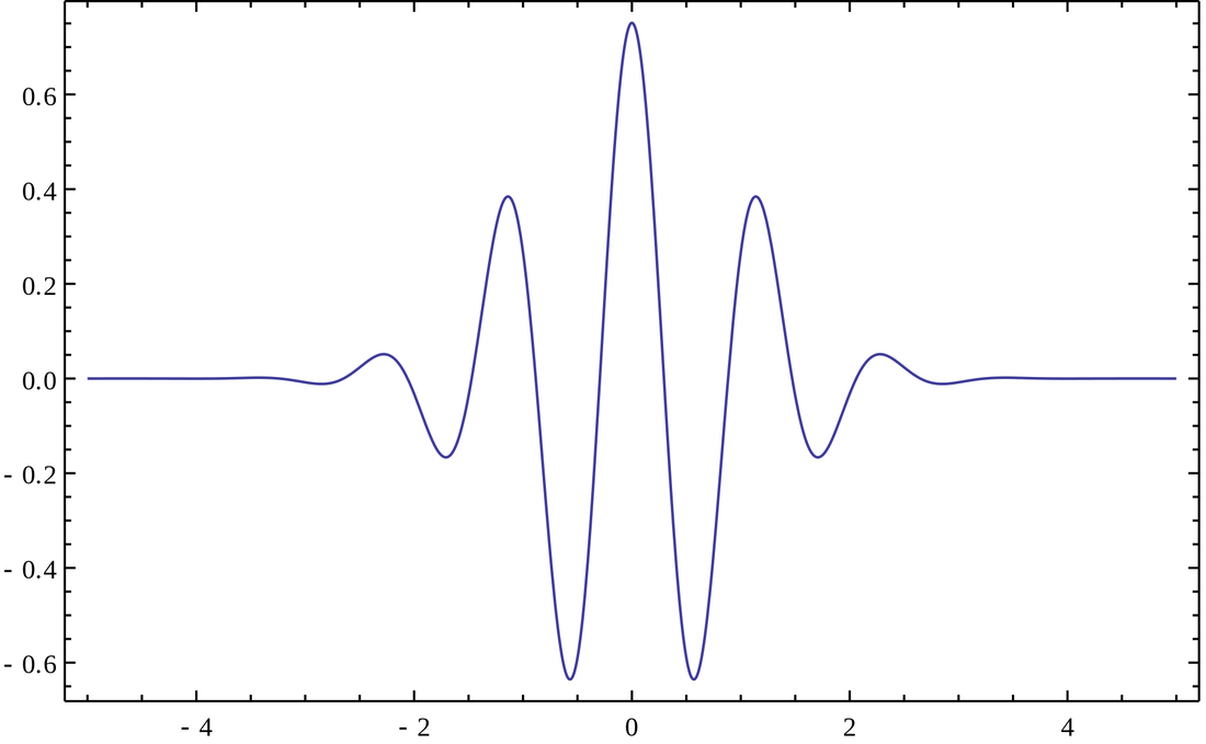
Morlet wavelet
Spectrogram:
The spectrogram is used to display the information of the intensity of a signal at specific time and specific frequency. It could show the result of our autotuned signal as well as the original signal, so we could know how well our autotune program work in frequency shifting.
Denoising:
Additive White Gaussian Noise (AWGN):
White Gaussian noise is a kind of noise that follows the same Gaussian distribution at all frequencies. As a result, they are random and have equal expectations of amplitude in all signals. This kind of noise will be generated by every electronic devices and cannot be eliminated physically.
White Gaussian noise is a kind of noise that follows the same Gaussian distribution at all frequencies. As a result, they are random and have equal expectations of amplitude in all signals. This kind of noise will be generated by every electronic devices and cannot be eliminated physically.
AWGN channel effect
Hard Thresholding vs. Soft Threashold:
The key to noise reduction is thresholding. We need to choose a property of the signal, decide a threshold, distinguish between noise and signal with regard to this threshold, then do something to eliminate noise and recover the signal. Roughly speaking, thresholding can be divided into hard thresholding and soft thresholding. Hard thresholding keeps those values that are larger than the threshold and makes those smaller than the threshold zero. Soft thresholding subtracts the threshold value from the original value and then makes all negative terms zero. Soft thresholding will keep the signal continuous after its work.
The key to noise reduction is thresholding. We need to choose a property of the signal, decide a threshold, distinguish between noise and signal with regard to this threshold, then do something to eliminate noise and recover the signal. Roughly speaking, thresholding can be divided into hard thresholding and soft thresholding. Hard thresholding keeps those values that are larger than the threshold and makes those smaller than the threshold zero. Soft thresholding subtracts the threshold value from the original value and then makes all negative terms zero. Soft thresholding will keep the signal continuous after its work.
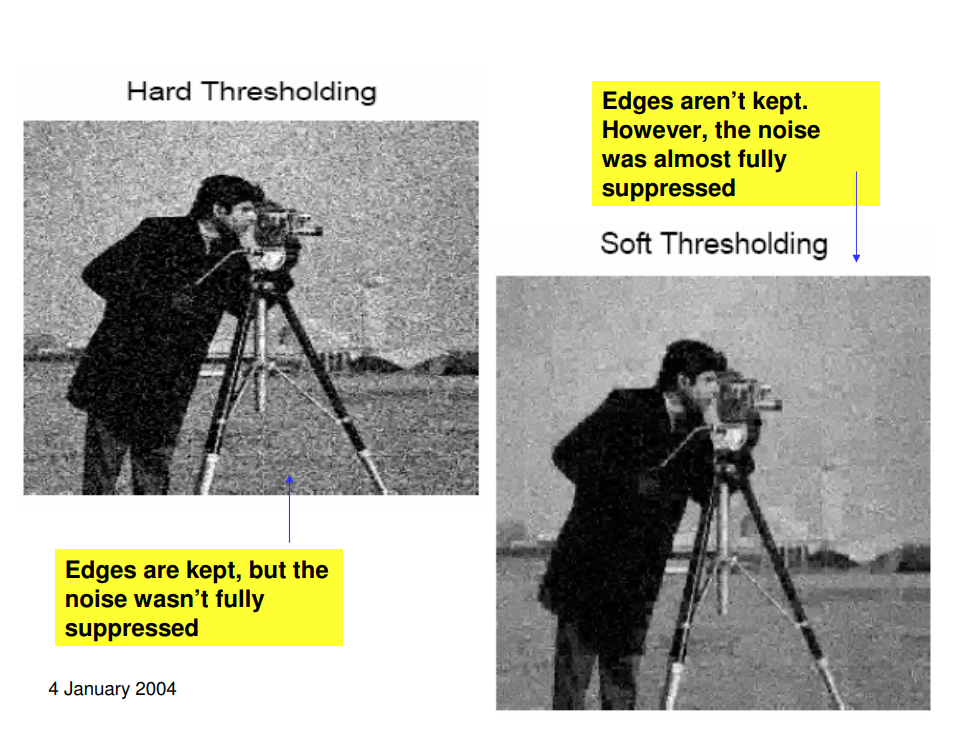
Hard thresholding vs Soft thresholding [6]
Block Thresholding:
Because the signal is not periodic, looking at the whole signal at once and choosing a threshold makes no sense. Therefore we divide the signal into small blocks and calculate threshold values for each block. This is called block thresholding.
Our Design:
We estimate SNR(dB) by applying the channel filter on a known constant signal and compare power before and after. The variance of the signal is calculated by
$$ \sigma_{v}^{2} \approx 10^{\frac{-S N R_{d B}}{10}} * \operatorname{var}(c[n]) $$ The noisy input signal can be represented by
$$ y[n]=x[n]+\epsilon[n] n=1,2 \ldots, N $$ where x[n] is the clean signal and \(\epsilon[n]\) is AWGN.
A wavelet transform coefficient of the noisy signal is $$ Y(a, b)=\sum_{n=1}^{N} y[n] \hat{\psi}\left(\frac{n-b}{a}\right) $$ The coefficients within one window are sorted in descending order by block length.
Our goal is to suppress noise. Therefore we need to first classify blocks into signal-dominant blocks where we will apply a loose threshold and noise-dominant blocks where we will apply a strict threshold. The classification is determined by the total power of the frame. If $$ \frac{1}{M} \sum_{k=1}^{M} S^{2}[k]>\sigma_{n}^{2} $$ it means that the average power of this block is greater than the expected power of the noise. We classify this block as signal-dominant. Otherwise, it is noise-dominant. Then we apply the following soft threshold: $$ \widetilde{X}[k]= \operatorname{sign}(S[k])\left[\max \left\{0, | S[k]-m_{s} k\right\}\right] if\ signal-dominant $$ $$ \widetilde{X}[k]= \operatorname{sign}(S[k])\left[\max \left\{0, | S[k]-m_{n} k\right\}\right] if\ noise-dominant $$ where m is a constant $$ m_{\mathrm{s}, n}=\frac{\lambda_{s, n} \sigma_{n}}{\frac{1}{M} \sum_{k=1}^{M} k^{2}} $$ \(\lambda_{s,n}\) controls the effect pf denoising. In general \(\lambda_s < \lambda_n\)
The denoised signal \(\widetilde{X}[k]\) will be fed into our auto-tuning programs.
Pitch Correction:
We tried many approaches to pitch correction. They can roughly be split based on whether or not there is a ground truth to compare to.
Phase-Vocoding Without Ground Truth
One approach we took to autotuning without a ground truth is a phase-vocoder method. This method starts by taking the STFT of the input signal. Then, the peaks in the STFT at each time are identified. This can be done by finding the points in the frequency spectrum which are larger than their two nearest neighbors on each side. Once the peaks are identified, the spectrum is segmented into regions of influence, which will move with the peaks when pitch correcting. This can be done in a number of ways. One method is to divide the region between adjacent peaks in half, putting the left half into the left peak's region of influence and the right half into the right peak's region of influence. Once regions of influence are determined, the peaks can be shifted, altered, deleted or duplicated as desired to adjust the pitch. When shifting the frequency of a peak, a phase-shift factor must be applied in order to preserve the audio quality. After multiplying by the phase-shift factor, an ISTFT (Inverse STFT) is applied to revert the signal to the time domain.
Phase-Vocoding has a number of distinct advantages. Because it uses an STFT and relies on simple identification and shifting of peaks, it is well-suited to real-time applications. Thus, phase-vocoding could be extremely useful for Auto-Tuning someone's voice in real time. Furthermore, finer manipulation of individual peaks in phase-vocoding can allow for automatic harmonization, chorusing, and manipulation of individual sounds in chords.
Phase-Vocoding also introduces some challenges because it can be difficult to determine how one should manipulate peaks. Peaks are introduced by the windowing function of the STFT as well as harmonics in sound recordings. It can often be challenging to determine how or which peaks should be shifted. In addition, if there is poor frequency resolution due to constraints on the windowing function for the STFT, then the sound quality can suffer significantly.
Thresholded Pitch-Shifting Without Ground Truth
Another approach we took to Auto-Tuning without a ground truth is to pitch-shift all frequencies above a certain threshold. First, we identify the frequencies whose component is above some fixed threshold. Then, we snap each of these frequencies individually to a table of pitches. This technique has the advantage of being very fast and simple, but the fixed threshold makes it hard to adapt to varying sound volumes. Additionally, this technique collapses the tips of peaks, potentially destroying some of the natural timbre of a sound. Lastly, it may sometimes be desirable to shift frequencies which fall below a certain threshold, but this depends on whether these sounds are noise or part of the true signal.
Auto-Tuning With Ground Truth
While Auto-Tuning with a ground truth can often be useful, if someone already has a set of target pitches (e.g. for a known, recorded song), they could try to fit the pitch of their singing to that ground truth. This is the core idea behind Auto-Tuning with a ground truth: take in a correct input and an incorrect input and shift the pitches of the incorrect input to match the correct input.
1. Column-wise
Iterate through each column of the spectrogram, find the blocks that have a value higher than a certain threshold, then rank the ground-truth and out-of-tune spectrogram according to the intensity. Then the out-of-tune spectrogram is tuned to the ground-truth spectrogram block by block in the order of ranking.
2. Segment-wise
Instead of iterating through all columns independently, the segment-wise algorithm first finds the syllable segments by searching for the great jumps in spectrogram intensity. After it has found the syllables, we tune each row in each segment to the closest ground truth spectrogram. This algorithm considers the time domain correlation, and is expected to generate less choppy results.
3. Pitch-wise
Segment-wise tuning still has the problem of ignoring the frequency domain correlation. So the third algorithm aims to find the entire pitch, and tune the pitches as an entity. In this way, the results should be much smoother and more natural than the other two algorithms.
4. Pitch Synchronous Overlap and Add (PSOLA)
PSOLA is a commonly used technique in DSP to modify pitch and duration. The algorithm first divides the audio signal into many windows, then it further divides each window into smaller overlapping segments.
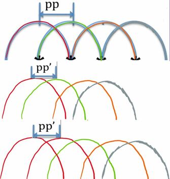
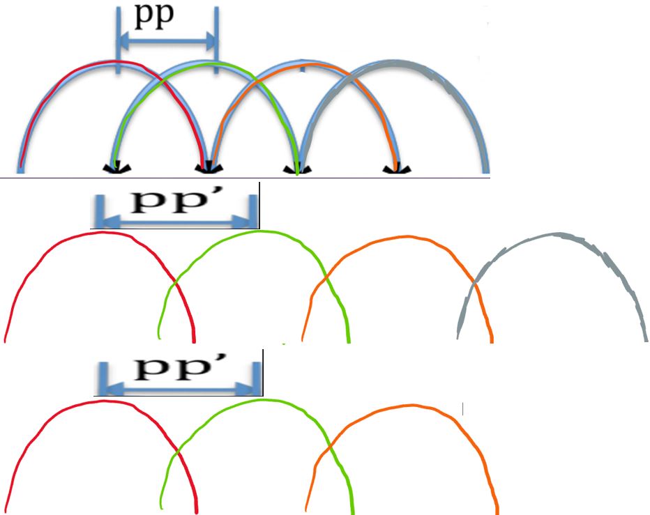
As shown in the picture below, to tune the frequency up, the segments are made closer by increasing the overlapping area. To remain the same duration, duplication of one segment in every N segments is performed.
Likewise, to tune the frequency down, the segments are set further apart, and partial segments are removed to make the duration still equal to the window's length.
Likewise, to tune the frequency down, the segments are set further apart, and partial segments are removed to make the duration still equal to the window's length.
|
|
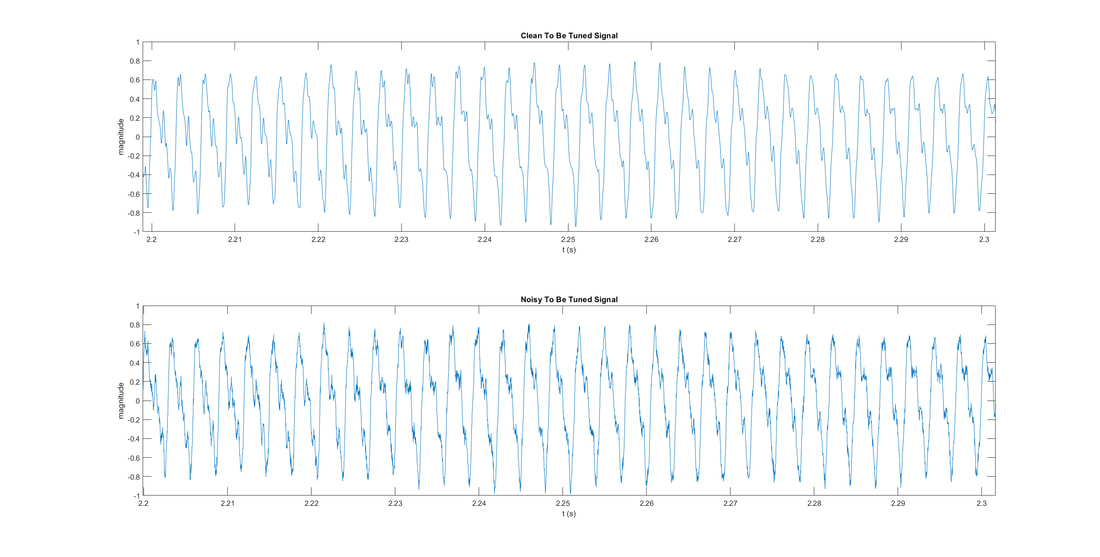
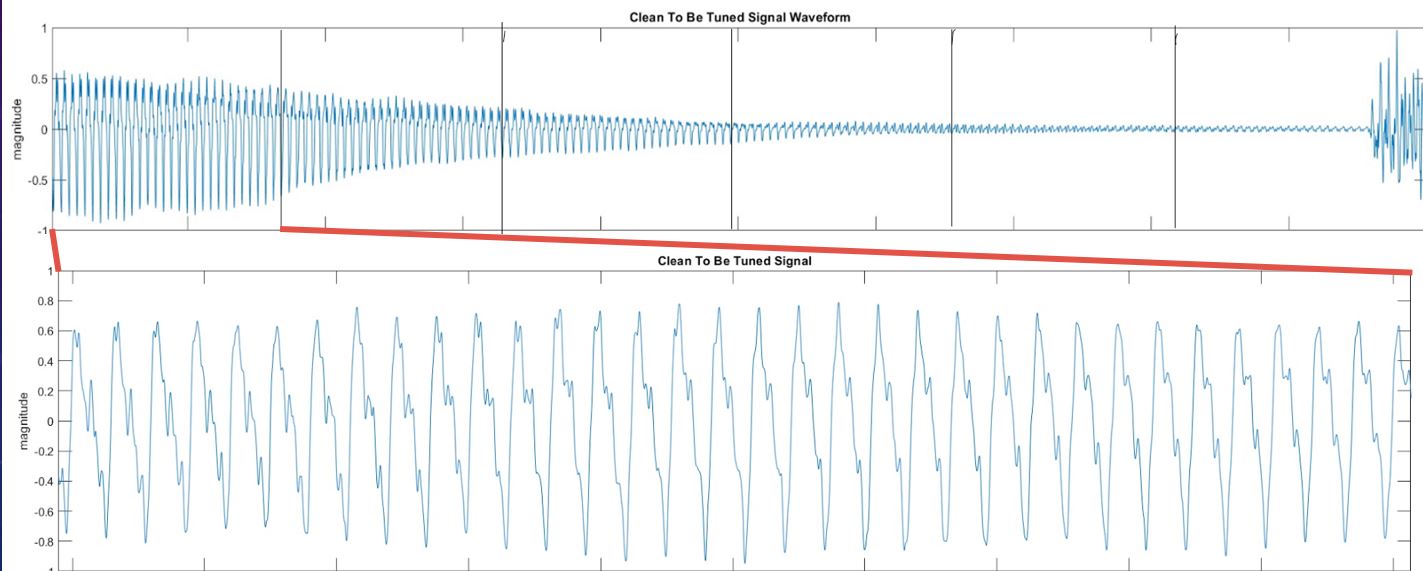
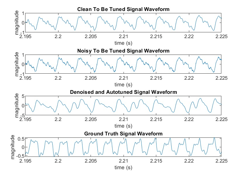
Below is the result of our PSOLA algorithm together with our denoising program. As you can see, the number of peaks of this signal segment is 10. After autotuning, the number of peaks increases to 13, which is equal to the number of peaks in the ground truth signal.
Smoothing:
Smoothing makes the tuned audio less awkward. Because (almost) no real-world music or songs are composed of totally discrete pitches, so transitions are need to make the audio sound more naturally. Smoothing is done by convolving a weighted mean filter to STFT coefficients.
Challenges
Frequency Detection:
- Our first challenge was window selection for the STFT. If we choose too large of a window, the time resolution becomes bad, and we will be unable to distinguish rapidly changing notes. If we choose too small of a window, the frequency resolution becomes bad, and we will be unable to distinguish low frequencies. For many of our experiments we stuck to a 1 second window, since it gave us the best audio quality for reasonable compute time.
- Determining pitches for a ground truth also proved to be difficult. We had to trade off between good frequency resolution and time resolution, as with window selection. We had trouble finding a good way of determining when the ground truth is changing pitch and when it is holding a pitch, and matching the target signal accordingly.
- Audio quality in general proved to be a problem. Some of our algorithms manipulated frequency components on a very fine-grained level, which damaged the timbre of our input sounds. To get cleaner sounds, we needed to use less fine-grained approaches, but these often did a poor job of identify primary frequencies.
Denoising:
- For block thresholding, the size of a block needs some consideration. If it is too large, it will mix two separate music notes together (in time or frequency) and then the threshold will not be very useful. If too small, the threshold cannot reflect the characteristics of the whole note it is in. Therefore this threshold is more likely to be inappropriate. We decided to make the block as small as possible in frequency (restricted by Wavelet Transform) and last 10ms.
- Audio with very low signal to noise ratio proved challenging to de-noise without damaging audio quality. This is expected since the noise is overpowering the signal. However, the highly structured nature of music should allow us to pick out musical signals with more advanced techniques in future work. For example, determining whether or not a note is being held and predicting future notes could help in identifying and clarifying a signal in the presence of noise.
Pitch Correction:
- When working without a ground truth, we are unable to do much better than moving a sound to the closest pitch. Sometimes this works, but if a note is very out of tune, this method fails.
- When pitch correcting, we often suffer from a trade off between having fine-grained control of each frequency in the spectrum and preserving the original timbre of the sound. More fine-grained control often gives better tuning results but can make the output sound almost unrecognizable.
- If multiple pitches are present in a track, our current implementations are unable to tune properly. It may be necessary to use advanced phase-vocoding techniques or other approaches to tune audio with multiple tracks.
Smoothing:
Without smoothing, our audio sounds very choppy. However, even with our current smoothing techniques, the output audio tracks often have unpleasant grinding or beating sounds in the background. This may require better smoothing techniques, although it may also arise from other things such as phase misalignment or too much modification of the frequency spectrum.